Special histograms in physt
Sometimes, it is necessary to bin values in transformed coordinates (e.g. polar). In principle, it is possible to create histograms from already transformed values (i.e. r and φ). However, this is not always the best way to go as each set of coordinates has its own peculiarities (e.g. the typical range of values for azimuthal angle)
Physt provides a general framework for constructing the transformed histograms (see a dedicated section of this document) and a couple of most frequently used variants:
PolarHistogram
SphericalHistogram
CylindricalHistogram
[1]:
# Necessary import evil
from physt import cylindrical, polar, spherical
import numpy as np
[2]:
# Generate some points in the Cartesian coordinates
np.random.seed(42)

x = np.random.rand(1000)
y = np.random.rand(1000)
z = np.random.rand(1000)
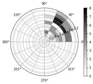
Polar histogram
This histograms maps values to radius (r) and azimuthal angle (φ, ranging from 0 to 2π).
By default (unless you specify the phi_bins parameter), the whole azimuthal range is spanned (even if there are no values that fall in parts of the circle).
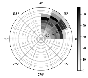
[3]:
# Create a polar histogram with default parameters
hist = polar(x, y)
ax = hist.plot.polar_map()
hist
[3]:
PolarHistogram(bins=(10, 16), total=1000, dtype=int64)
[4]:
hist.bins
[4]:
[array([[0.02704268, 0.16306851],
        [0.16306851, 0.29909433],
        [0.29909433, 0.43512015],
        [0.43512015, 0.57114597],
        [0.57114597, 0.7071718 ],
        [0.7071718 , 0.84319762],
        [0.84319762, 0.97922344],
        [0.97922344, 1.11524926],
        [1.11524926, 1.25127509],
        [1.25127509, 1.38730091]]),
 array([[0.        , 0.39269908],
        [0.39269908, 0.78539816],
        [0.78539816, 1.17809725],
        [1.17809725, 1.57079633],
        [1.57079633, 1.96349541],
        [1.96349541, 2.35619449],
        [2.35619449, 2.74889357],
        [2.74889357, 3.14159265],
        [3.14159265, 3.53429174],
        [3.53429174, 3.92699082],
        [3.92699082, 4.3196899 ],
        [4.3196899 , 4.71238898],
        [4.71238898, 5.10508806],
        [5.10508806, 5.49778714],
        [5.49778714, 5.89048623],
        [5.89048623, 6.28318531]])]
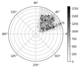
[5]:
# Create a polar histogram with different binning
hist2 = polar(x+.3, y+.3, radial_bins="pretty", phi_bins="pretty")
ax = hist2.plot.polar_map(density=True)
[6]:
# Default axes names
hist.axis_names
[6]:
('r', 'phi')
When working with any transformed histograms, you can fill values in the original, or transformed coordinates. All methods working with coordinates understand the parameter transformed which (if True) says that the method parameter are already in the transformed coordinated; otherwise, all values are considered to be in the original coordinates and transformed on inserting (creating, searching).
[7]:
# Using transformed / untransformed values
print("Non-transformed", hist.find_bin((0.1, 1)))
print("Transformed", hist.find_bin((0.1, 1), transformed=True))

print("Non-transformed", hist.find_bin((0.1, 2.7)))     # Value
print("Transformed", hist.find_bin((0.1, 2.7), transformed=True))
Non-transformed (7, 3)
Transformed (0, 2)
Non-transformed None
Transformed (0, 6)
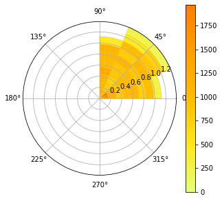
[8]:
# Simple plotting, similar to Histogram2D
hist.plot.polar_map(density=True, show_zero=False, cmap="Wistia", lw=0.5, figsize=(5, 5));
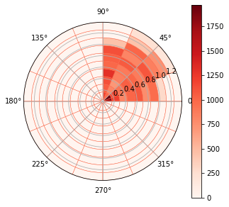
Adding new values
[9]:
# Add a single, untransformed value
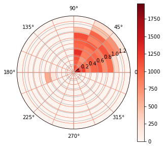
hist.fill((-.5, -.5), weight=12)
hist.plot.polar_map(density=True, show_zero=True, cmap="Reds", lw=0.5, figsize=(5, 5));
[10]:
# Add a couple of values, transformed
data = [[.5, 3.05], [.5, 3.2], [.7, 3.3]]
weights = [1, 5, 20]

hist.fill_n(data, weights=weights, transformed=True)
hist.plot.polar_map(density=True, show_zero=True, cmap="Reds", lw=0.5, figsize=(5, 5));
Projections
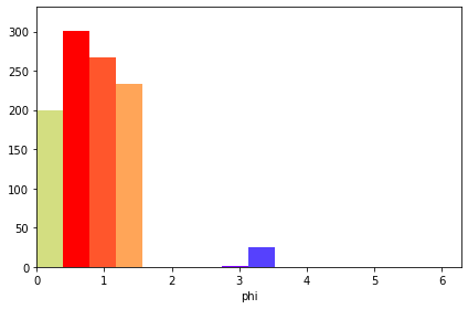
The projections are stored using specialized Histogram1D subclasses that keep (in the case of radial) information about the proper bin sizes.
[11]:
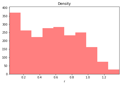
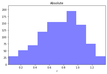
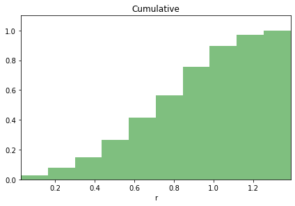
radial = hist.projection("r")
radial.plot(density=True, color="red", alpha=0.5).set_title("Density")
radial.plot(label="absolute", color="blue", alpha=0.5).set_title("Absolute")
radial.plot(label="cumulative", cumulative=True, density=True, color="green", alpha=0.5).set_title("Cumulative")
radial
[11]:
RadialHistogram(bins=(10,), total=1026, dtype=int64)
[12]:
hist.projection("phi").plot(cmap="rainbow")
[12]:
<Axes: xlabel='phi'>
Cylindrical histogram
To be implemented
[13]:
data = np.random.rand(100, 3)
h = cylindrical(data)
h
[13]:
CylindricalHistogram(bins=(10, 16, 10), total=100, dtype=int64)
[14]:
# %matplotlib qt
proj = h.projection("rho", "phi")
proj.plot.polar_map()
proj
[14]:
PolarHistogram(bins=(10, 16), total=100, dtype=int64)
[15]:
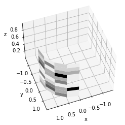
proj = h.projection("phi", "z")
ax = proj.plot.cylinder_map(show_zero=False)
ax.view_init(50, 70)
proj
[15]:
CylindricalSurfaceHistogram(bins=(16, 10), total=100, dtype=int64)
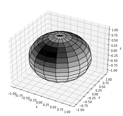
Spherical histogram
To be implemented
[16]:
n = 1000000
data = np.empty((n, 3))
data[:,0] = np.random.normal(0, 1, n)
data[:,1] = np.random.normal(0, 1.3, n)
data[:,2] = np.random.normal(1, 1.2, n)
h = spherical(data)
h
[16]:
SphericalHistogram(bins=(10, 16, 16), total=1000000, dtype=int64)
[17]:
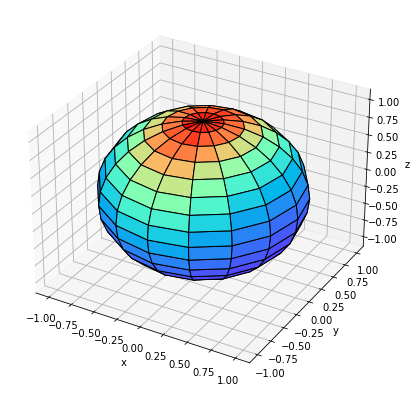
globe = h.projection("theta", "phi")
# globe.plot()
globe.plot.globe_map(density=True, figsize=(7, 7), cmap="rainbow")
globe.plot.globe_map(density=False, figsize=(7, 7))
globe
[17]:
SphericalSurfaceHistogram(bins=(16, 16), total=1000000, dtype=int64)
Implementing custom transformed histogram
TO BE WRITTEN